Mathematics And Theory Behind The Magic of Linear Regression

Introduction 

"Machine learning is the new electricity", is something which we have heard once in our lifetime. From the use of photos app to social media  there is some use of it in almost every aspect of our day to day life. Today lets look at one of the basic machine learning algorithm which almost anyone can learn and use to predict new outcomes of linear data.

Before moving on to the actual algorithm lets give a quick look at high school maths which many of us may remember. 

• The equation of a straight line : Y = mx +b 

• The distance between two points(x₁,y₁ and x₂,y₂)  = √(x₂-x₁)²+(y₂-y₁)²

What is Linear Regression?

Linear regression is a regression algorithm to find a best fitting line to the given linearly related data-set. Such data set could be the house price with house features or could be as simple as the marks obtained by a student per hours they invest in their studies. Lets visualize a data set where we plot the students marks with the number of hours they invest in their studies. Please notice this is a test score with full marks of 120 and not 100 as we have.

Objective of problem

The objective of the linear regression problem is to find a best fitting line which has a minimum distance from all the given points in the given data set. After reading this blog you will be able to draw a line in the given data set which we will call the best fitting line.

How do we start?

Well, this is the easiest part of the algorithm, we start with a random value or zero value of slope(m) and the bias or y-intercept(b) then we find the error(cost) of the line then we make a slight tweak to m and b and again repeat this process until we have converge to minimum error. In machine learning terms we can call this function which we use to predict as a hypothesis and in the case of linear regression we have our hypothesis : ŷ = mx+b

What is the cost function?

The cost function is the function will give us the error in our hypothesis or prediction line. We will be using the mean squared error cost function for this problem. In the squared error cost function, we calculate the distance between the actual score of students and our predicted score. For a single training example at hour of study = 30, if the prediction is 20 and the actual value is 40 then we can say our error is the distance between them which will be,

    error = (ŷ - y)² =(20-40)² = 400

The actual cost function is the mean of all the errors in our training examples. lets denote cost function with J(ŷ,y), then 

J(ŷ,y) = 1/2M * ∑ (ŷ - y) ²

where M is the number of training examples.

This is the cost function which will calculate the mean of squared error from our predicted hypothesis and the actual value.

The objective of the linear regression is to minimize this cost function. To gain more intuition about the cost function lets look at its graph where we plot slope in x axis , bias in y axis and cost function in the z axis.

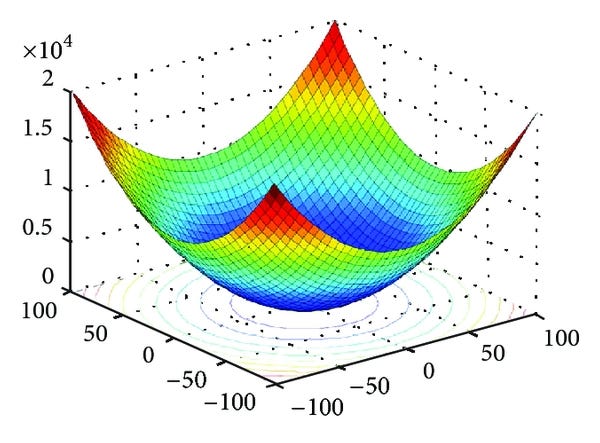
image source: Medium

Here we can see that with optimum values of m and b we can minimize this function and the way we minimize this function is called optimization algorithm.

Optimization algorithm

When it comes to optimization algorithm there are many we have but the easiest and most intuitive one I have found is the gradient descent optimization algorithm. Before looking at the algorithm itself lets have a look at how the gradient descent will converge to the minimum value with this video from medium.

image source : medium

As we can see, the values of m and b are tweaked such that they reach the local minimum and it does it by using this algorithm. The values of m and b are updated as follows:

That is a lot of maths and calculus but I will not bore you with the proof of the partial derivatives. But a thing to notice is that there is a introduction of a new variable called the learning rate which is denoted by alpha. The value of alpha depends upon the data set and its optimum value can be gathered by hit and trail method or taking a value and dividing or multiplying it by 3 as per the outcome we get. Usually we start with value as 0.0001 and if it tries to converge to minimum value but overshoots then we divide it by 3 then try again or else if it converges too slow then we can try to multiply it again and try it.

The small tweaking of the learning rate * partial derivative will help the m and b move down the slope to the minimum as shown in the gif above.

Conclusion

So, In this way we can find the optimum value for our parameters m and b to make it best fitting line. The thing to remember that the gradient step is very small step so we may need to tweak the values of m and b for multiple times usually 1000 to 10000. That seems like a lot of computation but thanks to computers we can write small lines of codes to do this task for such large number of times within seconds. In the next blog I will be posting a python version of this codes to help you build a linear regression from scratch and make predictions on linear data.