Mathematics And Theory Behind The Magic of Logistic Regression

Introduction

Is that a bird? Is that a plane? Well, ask no more, we  have just got the algorithm which can classify the given input into a label or as we denote them as 0 or 1, 0 standing for a no and 1 for yes and it is called logistic regression.

But why Logistic Regression?

In previous blog I shared a basic idea about linear regression and while linear regression can be a great tool for linearly related data but when it comes to classification it is not quite useful because we need to come up with a non linear way to give our result and logistic regression is just about it.

Where do we want to use logistic regression?

The area of logistic regression is classification. By looking at the entrance marks of a student we can classify whether s/he may get selected or not, by looking at the size of tumor we can classify whether it is malignant or not. The possibilities are endless but lets look at why will linear regression fail to converge in such data set.

The line y = mx+b is not the best ideal fit for the data set so lets look at logistic function or a sigmoid function.

image source : Wikipedia

As we can see this is a sigmoid or a logistic function has value ranging from 0 to one and if we can find the optimum value of the weights for X and bias then we can fit our data set to give accurate predictions( we will talk more about this below) but first lets talk about the sigmoid function.

This is a sigmoid function which will always give us a value in between 0 and 1.

Just passing x as input we will not be able to train and converge anything so we will multiply x with weight W and add bias b which we will be using to train the features. 

What are weights and bias?

Just like in the linear regression we trained slope and y intercept to get the best fitting line here in logistic regression I introduce you to the weights and bias. Weights and bias are number or more than number they are a matrix of numbers which will help us predict either zero or one. Our hypothesis will be slightly changed as follows:

ŷ = σ(ώx+b)

where sigma (σ) is sigmoid function and ώ is the transpose of W matrix.

What if the inputs have multiple features?

Till now we have only discussed if input or X has only one feature that is in case of our data set only one input which is the size of tumor is given but we may have multiple features as our inputs. For example, if we are making a prediction whether a person will be able to survive from corona virus then we may need to look at multiple features of that person like blood pressure, sugar level, kidney problems, heart health, recent surgeries etc. and after analysis of such data only we can  say whether the person will survive(y=1) or will not survive(y=0). In such case X will be a vector of dimension (n,M) where n is the number of features. Then W should also be a vector of dimension (n,1) then the dot product of W transpose with x will give a scalar value which we can add the bias to and send it to the sigmoid function. We can represent this process in a simple figure which will help us gain more intuition.

The initial values for the weights and bias is zero and then we tweak some values in them to get to minimum error, but hey what is the cost function to be used?

Cost Function

For the logistic regression we don't use the mean squared error cost function because it may have multiple minimum and  may converge to a local minimum instead of a global minimum.

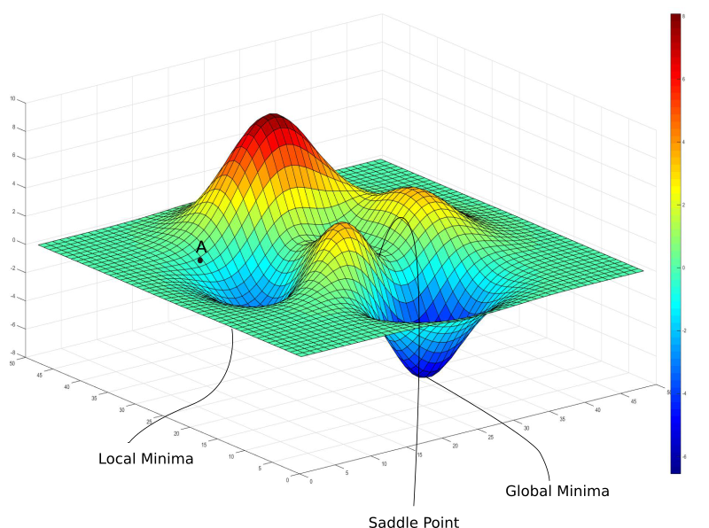
image source : paperspace

So we need to come up with a better cost function J(ŷ,y)

J(ŷ,y) = - 1/M * Σ y log(ŷ) + (1-y) log (1-ŷ)

Here log is the natural logarithm and not logarithm with base 10.  

On expansion of ŷ the cost function becomes:

J = -1/M * ∑ y log(σ(ώx + b)) + (1-y)  log(1 - σ(ώx + b))

where σ is the sigmoid or logistic function.

Optimization Algorithm 

Similar to linear regression there is use of gradient descent algorithm to converge the values of W and b to the global minimum. Yes, we can use other famous optimization algorithms like stochastic gradient descent , adam etc. but gradient descent is easy to understand for a high school student with basic calculus knowledge. Similar to linear regression we take the partial derivative of the cost function with respect to weight and then with respect to bias and the subtract weights and bias with the derivative(slope) multiplied to a parameter called the learning rate, mathematically speaking the algorithm will look like this :

The handwriting is a bit sloppy but hey we need some slopes to get optimized to minimum errors.

The value of alpha(learning) is not just a parameter it is a hyper parameter which will determine whether the function will converge or not so while choosing it we should be careful, the usual value ranges from 0.01 to 0.0001. By repeating this process for multiple times we can converge the values of W and b which can be later used to give predictions on new data.

image source: medium

Conclusion

So, by now you have gained all the knowledge and intuition about logistic regression, this can be used to classify either the given picture is dog or cat, whether the person will die of corona virus, whether the tumor is malignant or not and endless possibilities of questions which has a yes or no can be used to classified with logistic regression, next I will talk about Artificial Neural Networks (ANN) and share some jupyter(yes that is the correct spelling of jupyter ) notebooks of python code where I will be sharing ideas on linear regression, logistic regression, and artificial neural networks.